Previous research has shown that modern Eurasians interbred with their Neanderthal and Denisovan predecessors. We show here that hundreds of thousands of years earlier, the ancestors of Neanderthals and Denisovans interbred with their own Eurasian predecessors—members of a “superarchaic” population that separated from other humans about 2 million years ago. The superarchaic population was large, with an effective size between 20 and 50 thousand individuals. We confirm previous findings that (i) Denisovans also interbred with superarchaics, (ii) Neanderthals and Denisovans separated early in the middle Pleistocene, (iii) their ancestors endured a bottleneck of population size, and (iv) the Neanderthal population was large at first but then declined in size. We provide qualified support for the view that (v) Neanderthals interbred with the ancestors of modern humans.
INTRODUCTION
During the past decade, we have learned about interbreeding among hominin populations after 50 thousand years (ka) ago, when modern humans expanded into Eurasia (1–3). Here, we focus farther back in time, on events that occurred more than a half million years ago. In this earlier time period, the ancestors of modern humans separated from those of Neanderthals and Denisovans. Somewhat later, Neanderthals and Denisovans separated from each other. The paleontology and archaeology of this period record important changes, as large-brained hominins appear in Europe and Asia and Acheulean tools appear in Europe (4, 5). It is not clear, however, how these large-brained hominins relate to other populations of archaic or modern humans (6–9). We studied this period using genetic data from modern Africans and Europeans and from two archaic populations, Neanderthals and Denisovans.
Figure 1 illustrates our notation. Uppercase letters refer to populations, and combinations such as XY refer to the population ancestral to X and Y. X represents an African population (the Yorubans), Y is a European population, N is Neanderthals, and D is Denisovans. S is an unsampled “superarchaic” population that is distantly related to other humans. Lowercase letters at the bottom of Fig. 1 label “nucleotide site patterns.” A nucleotide site exhibits site pattern xyn if random nucleotides from populations X, Y, and N carry the derived allele, but those sampled from other populations are ancestral. Site pattern probabilities can be calculated from models of population history, and their frequencies can be estimated from data. Our Legofit (10) software estimates parameters by fitting models to these relative frequencies.
<a href=”https://advances.sciencemag.org/content/advances/6/8/eaay5483/F1.large.jpg?width=800&height=600&carousel=1″ title=”A population network including four episodes of gene flow, with an embedded gene genealogy. Upper case letters (X, Y, N, D, and S) represent populations (Africa, Europe, Neanderthal, Denisovan, and superarchaic). Greek letters label episodes of admixture. d and xyn illustrate two nucleotide site patterns, in which 0 and 1 represent the ancestral and derived alleles. A mutation on the red branch would generate site pattern d. One on the blue branch would generate xyn. For simplicity, this figure refers to Neanderthals with a single letter. Elsewhere, we use two letters to distinguish between the Altai and Vindija Neanderthals.” class=”fragment-images colorbox-load” rel=”gallery-fragment-images-1908649491″ data-figure-caption=”
Fig. 1A population network including four episodes of gene flow, with an embedded gene genealogy.
Upper case letters (X, Y, N, D, and S) represent populations (Africa, Europe, Neanderthal, Denisovan, and superarchaic). Greek letters label episodes of admixture. d and xyn illustrate two nucleotide site patterns, in which 0 and 1 represent the ancestral and derived alleles. A mutation on the red branch would generate site pattern d. One on the blue branch would generate xyn. For simplicity, this figure refers to Neanderthals with a single letter. Elsewhere, we use two letters to distinguish between the Altai and Vindija Neanderthals.
” data-icon-position data-hide-link-title=”0″>
Fig. 1A population network including four episodes of gene flow, with an embedded gene genealogy.
Upper case letters (X, Y, N, D, and S) represent populations (Africa, Europe, Neanderthal, Denisovan, and superarchaic). Greek letters label episodes of admixture. d and xyn illustrate two nucleotide site patterns, in which 0 and 1 represent the ancestral and derived alleles. A mutation on the red branch would generate site pattern d. One on the blue branch would generate xyn. For simplicity, this figure refers to Neanderthals with a single letter. Elsewhere, we use two letters to distinguish between the Altai and Vindija Neanderthals.
Nucleotide site patterns contain only a portion of the information available in genome sequence data. This portion, however, is of particular relevance to the study of deep population history. Site pattern frequencies are unaffected by recent population history because they ignore the within-population component of variation (10). This reduces the number of parameters we must estimate and allows us to focus on the distant past.
The current data include two high-coverage Neanderthal genomes: one from the Altai Mountains of Siberia and the other from Vindija Cave in Croatia (11). Rather than assigning the two Neanderthal fossils to separate populations, our model assumes that they inhabited the same population at different times. This implies that our estimates of Neanderthal population size will refer to the Neanderthal metapopulation rather than to any individual subpopulation.
The Altai and Vindija Neanderthals appear in site pattern labels as “a” and “v”. Thus, av is the site pattern in which the derived allele appears only in nucleotides sampled from the two Neanderthal genomes. Figure 2 shows the site pattern frequencies studied here. In contrast to our previous analysis (12), the current analysis includes singleton site patterns, x, y, v, a, and d, as advocated by Mafessoni and Prüfer (13). A simpler tabulation, which excludes the Vindija genome, is included as fig. S2.
<a href=”https://advances.sciencemag.org/content/advances/6/8/eaay5483/F2.large.jpg?width=800&height=600&carousel=1″ title=”Observed site pattern frequencies. Horizontal axis shows the relative frequency of each site pattern in random samples consisting of a single haploid genome from each of X, Y, V, A, and D, representing Africa, Europe, Vindija Neanderthal, Altai Neanderthal, Denisovan, and superarchaic. Horizontal lines (which look like dots) are 95% confidence intervals estimated by a moving blocks bootstrap (35). Data: Simons Genome Diversity Project (SGDP) (14) and Max Planck Institute for Evolutionary Anthropology (11).” class=”fragment-images colorbox-load” rel=”gallery-fragment-images-1908649491″ data-figure-caption=”
Fig. 2Observed site pattern frequencies.
Horizontal axis shows the relative frequency of each site pattern in random samples consisting of a single haploid genome from each of X, Y, V, A, and D, representing Africa, Europe, Vindija Neanderthal, Altai Neanderthal, Denisovan, and superarchaic. Horizontal lines (which look like dots) are 95% confidence intervals estimated by a moving blocks bootstrap (35). Data: Simons Genome Diversity Project (SGDP) (14) and Max Planck Institute for Evolutionary Anthropology (11).
” data-icon-position data-hide-link-title=”0″>
Fig. 2Observed site pattern frequencies.
Horizontal axis shows the relative frequency of each site pattern in random samples consisting of a single haploid genome from each of X, Y, V, A, and D, representing Africa, Europe, Vindija Neanderthal, Altai Neanderthal, Denisovan, and superarchaic. Horizontal lines (which look like dots) are 95% confidence intervals estimated by a moving blocks bootstrap (35). Data: Simons Genome Diversity Project (SGDP) (14) and Max Planck Institute for Evolutionary Anthropology (11).
Greek letters in Fig. 1 label episodes of admixture. We label models by concatenating Greek letters to indicate the episodes of admixture they include. For example, model “αβ” includes only episodes α and β. Our model does not include gene flow from Denisovans into moderns because there is little evidence of such gene flow into Europeans (14, 15). Two years ago, we studied a model that included only one episode of admixture: α, which refers to gene flow from Neanderthals into Europeans (12). The left panel of Fig. 3 shows the residuals from this model, using the new data. Several are far from zero, suggesting that something is missing from the model (16).
<a href=”https://advances.sciencemag.org/content/advances/6/8/eaay5483/F3.large.jpg?width=800&height=600&carousel=1″ title=”Residuals from models α and αβγδ. Key: red asterisks, real data; blue circles, 50 bootstrap replicates.” class=”fragment-images colorbox-load” rel=”gallery-fragment-images-1908649491″ data-figure-caption=”
Fig. 3Residuals from models α and αβγδ.
Key: red asterisks, real data; blue circles, 50 bootstrap replicates.
” data-icon-position data-hide-link-title=”0″>
Fig. 3Residuals from models α and αβγδ.
Key: red asterisks, real data; blue circles, 50 bootstrap replicates.
Recent literature suggests some of what might be missing. There is evidence for admixture into Denisovans from a superarchaic population, which was distantly related to other humans (2, 11, 17–19), and also for admixture from early moderns into Neanderthals (19). These episodes of admixture appear as β and γ in Fig. 1. Adding β and/or γ to the model improved the fit, yet none of the resulting models were satisfactory. For example, model αβγ implied (implausibly) that superarchaics separated from other hominins 7 million years (Ma) ago.
To understand what might still be missing, consider what we know about the early middle Pleistocene, around 600 ka ago. At this time, large-brained hominins appear in Europe, along with Acheulean stone tools (4, 5). They were probably African immigrants, because similar fossils and tools occur earlier in Africa. According to one hypothesis, these early Europeans were Neanderthal ancestors (6, 7). Somewhat earlier—perhaps 750 ka ago [(8), table S12.2]—the “neandersovan” ancestors of Neanderthals and Denisovans separated from the lineage leading to modern humans. Neandersovans may have separated from an African population and then expanded into Eurasia. If so, then they would not have been expanding into an empty continent, for Eurasia had been inhabited since 1.85 Ma ago (20). Neandersovan immigrants may have met the indigenous superarchaic population of Eurasia. This suggests a fourth episode of admixture, from superarchaics into neandersovans, which appears as δ in Fig. 1.
RESULTS
We considered eight models, all of which include α, and including all combinations of β, γ, and/or δ. In choosing among complex models, it is important to avoid overfitting. Conventional methods such as Akaike’s information criterion (21) are not available because we do not have access to the full likelihood function. Instead, we use the bootstrap estimate of predictive error (bepe) (10, 22, 23). The best model is the one with the lowest value of bepe. When no model is clearly superior, it is better to average across several than to choose just one (24). For this purpose, we used bootstrap model averaging (booma) (10, 24). The booma weight of the ith model is the fraction of datasets (including the real data and 50 bootstrap replicates) in which that model “wins,” i.e., has the lowest value of bepe. The bepe values and booma weights of all models are in Table 1.
Table 1bepe values and booma weights.
View this table:
The best model is αβγδ, which includes all four episodes of admixture. It has smaller residuals (Fig. 3, right), the lowest bepe value, and the largest booma weight. One other model, αβδ, has a positive booma weight, but all others have zero weight. To understand what this means, recall that bootstrap replicates approximate repeated sampling from the process that generated the data. The models with zero weight lose in all replicates, implying that their disadvantage is large compared with variation in repeated sampling. On this basis, we can reject these models. Neither of the two remaining models can be rejected. These results provide strong support for two episodes of admixture (β and δ) and qualified support for a third (γ). Not only does this support previously reported episodes of gene flow but it also reveals a much older episode, in which neandersovans interbred with superarchaics. Model-averaged parameter estimates, which use the weights in Table 1, are graphed in Fig. 4 and listed in table S1.
<a href=”https://advances.sciencemag.org/content/advances/6/8/eaay5483/F4.large.jpg?width=800&height=600&carousel=1″ title=”Model-averaged parameter estimates with 95% confidence intervals estimated by moving blocks bootstrap (35). Key: mα, fraction of Y introgressed from N; mβ, fraction of D introgressed from S; mγ, fraction of N introgressed from XY; mδ, fraction of ND introgressed from S; TXYNDS, superarchaic separation time; TXY, separation time of X and Y; TND, separation time of N and D; TN0, end of early epoch of Neanderthal history; TA, age of Altai Neanderthal fossil; TV, age of Vindija Neanderthal fossil; TD, age of Denisovan fossil; NS, size of superarchaic population; NXYND, size of populations XYND and XYNDS; NXY, size of population XY; NND, size of population ND; NN0, size of early Neanderthal population; NN1, size of late Neanderthal population. Parameters that exist in only one model are not averaged.” class=”fragment-images colorbox-load” rel=”gallery-fragment-images-1908649491″ data-figure-caption=”
Fig. 4Model-averaged parameter estimates with 95% confidence intervals estimated by moving blocks bootstrap (35).
Key: mα, fraction of Y introgressed from N; mβ, fraction of D introgressed from S; mγ, fraction of N introgressed from XY; mδ, fraction of ND introgressed from S; TXYNDS, superarchaic separation time; TXY, separation time of X and Y; TND, separation time of N and D; TN0, end of early epoch of Neanderthal history; TA, age of Altai Neanderthal fossil; TV, age of Vindija Neanderthal fossil; TD, age of Denisovan fossil; NS, size of superarchaic population; NXYND, size of populations XYND and XYNDS; NXY, size of population XY; NND, size of population ND; NN0, size of early Neanderthal population; NN1, size of late Neanderthal population. Parameters that exist in only one model are not averaged.
” data-icon-position data-hide-link-title=”0″>
Fig. 4Model-averaged parameter estimates with 95% confidence intervals estimated by moving blocks bootstrap (35).
Key: mα, fraction of Y introgressed from N; mβ, fraction of D introgressed from S; mγ, fraction of N introgressed from XY; mδ, fraction of ND introgressed from S; TXYNDS, superarchaic separation time; TXY, separation time of X and Y; TND, separation time of N and D; TN0, end of early epoch of Neanderthal history; TA, age of Altai Neanderthal fossil; TV, age of Vindija Neanderthal fossil; TD, age of Denisovan fossil; NS, size of superarchaic population; NXYND, size of populations XYND and XYNDS; NXY, size of population XY; NND, size of population ND; NN0, size of early Neanderthal population; NN1, size of late Neanderthal population. Parameters that exist in only one model are not averaged.
Episode δ, which proposes gene flow from superarchaics into neandersovans, is a novel hypothesis. Before accepting it, we should ask whether the evidence in its favor could be artifactual, reflecting a bias in site pattern frequencies caused by sequencing error or somatic mutations. Sequencing error adds a positive bias to the frequency of each singleton site pattern proportional to the per-nucleotide error rate in the corresponding population (see the Supplementary Materials). Somatic mutations have a similar effect. These biases might explain evidence for episode δ, if it were true that larger values of mδ (the fraction of superarchaic admixture in neandersovans) imply larger frequencies of singleton site patterns. However, Table 2 shows that this is not the case. There is no consistent tendency for singleton frequencies to increase with mδ. Indeed, three of them decrease. Consequently, evidence that mδ > 0 cannot be the result of a positive bias in the frequencies of singleton site patterns. The evidence for δ admixture cannot be an artifact of sequencing error or somatic mutations.
Table 2Effect on singleton site pattern frequencies of gene flow (mδ) from superarchaics into neandersovans.
Column 2 shows expected frequencies of singleton site patterns in a model in which mδ = 0, and all other parameters are as fitted under model αβγδ. In column 3, all parameters including mδ are as fitted under this model. Column 4 is obtained by subtracting column 2 from column 3. Expected site pattern frequencies were estimated using legosim with 107 iterations.
View this table:
The superarchaic separation time, TXYNDS, has a point estimate of 2.3 Ma ago. This estimate may be biased upward because our molecular clock assumes a fairly low mutation rate of 0.38 × 10⁻⁹ per nucleotide site per year. Other authors prefer slightly higher rates (25). Although this rate is apparently insensitive to generation time among the great apes, it is sensitive to the age of male puberty. If the average age of puberty during the past 2 Ma were halfway between those of modern humans and chimpanzees, the yearly mutation rate would be close to 0.45 × 10⁻⁹ [(26), Fig. 2B], and our estimate of TXYNDS would drop to 1.9 Ma, just at the origin of the genus Homo. Under this clock, the 95% confidence interval is 1.8 to 2.2 Ma.
If superarchaics separated from an African population, then this separation must have preceded the arrival of superarchaics in Eurasia. Nonetheless, our 1.8 to 2.2 Ma interval includes the 1.85 Ma date of the earliest Eurasian archaeological remains at Dmanisi (20). Thus, superarchaics may descend from the earliest human dispersal into Eurasia, as represented by the Dmanisi fossils. On the other hand, some authors prefer a higher mutation rate of 0.5 × 10⁻⁹ per year (2). Under this clock, the lower end of our confidence interval would be 1.6 Ma ago. Thus, our results are also consistent with the view that superarchaics entered Eurasia after the earliest remains at Dmanisi.
Parameter NS is the effective size of the superarchaic population. This parameter can be estimated because there are two sources of superarchaic DNA in our sample (β and δ), and this implies that coalescence time within the superarchaic population affects site pattern frequencies. Although this parameter has a broad confidence interval, even the low end implies a fairly large population of about 20,000. This does not require large numbers of superarchaic humans, because effective size can be inflated by geographic population structure (27). Our large estimate may mean that neandersovans and Denisovans received gene flow from two different superarchaic populations.
Parameter TND is the separation time of Neanderthals and Denisovans. Our point estimate, 737 ka ago, is remarkably old. Furthermore, the neandersovan population that preceded this split was remarkably small: NND ≈ 500. This supports our previous results, which indicated an early separation of Neanderthals and Denisovans and a bottleneck among their ancestors (12).
Because our analysis includes two Neanderthal genomes, we can estimate the effective size of the Neanderthal population in two separate epochs. The early epoch extends from TN0 = 455 ka to TND = 737 ka, and within this epoch, the effective size was large: NN0 ≈ 16,000. It was smaller during the later epoch: NN1 ≈ 3400. These results support previous findings that the Neanderthal population was large at first but then declined in size (2, 11).
DISCUSSION
This project began with a puzzle. We had argued in 2017 that Neanderthals and Denisovans separated early, that their neandersovan ancestors endured a bottleneck of population size, and that the postseparation Neanderthal population was large (12). That analysis omitted singleton site patterns. Mafessoni and Prüfer (13) pointed out that introducing singletons led to different results. In response, Rogers et al. (16) agreed, but also observed that the with-singleton analysis implied that the Denisovan fossil was only 4000 years old—a result that is plainly wrong. Furthermore, a residual analysis showed that neither of the models under discussion in 2017 fit the data very well (16). Something was apparently missing from both models—but what? The present paper provides an answer to that question.
Our results shed light on the early portion of the middle Pleistocene, about 600 ka ago, when large-brained hominins appear in the fossil record of Europe along with Acheulean stone tools. There is disagreement about how these early Europeans should be interpreted. Some see them as the common ancestors of modern humans and Neanderthals (28), others as an evolutionary dead end, later replaced by immigrants from Africa (29, 30), and others as early representatives of the Neanderthal lineage (6, 7). Our estimates are most consistent with the last of these views. They imply that by 600 ka ago, Neanderthals were already a distinct lineage, separate not only from the modern lineage but also from Denisovans.
These results resolve a discrepancy involving human fossils from Sima de los Huesos (SH). Those fossils had been dated to at least 350 ka ago and perhaps 400 to 500 ka ago (31). Genetic evidence showed that they were from a population ancestral to Neanderthals and therefore more recent than the separation of Neanderthals and Denisovans (9). However, genetic evidence also indicated that this split occurred about 381 ka ago [(2), table S12.2]. This was hard to reconcile with the estimated age of the SH fossils. To make matters worse, improved dating methods later showed that the SH fossils are even older, about 600 ka, and much older than the molecular date of the Neanderthal-Denisovan split (32). Our estimates resolve this conflict because they push the date of the split back well beyond the age of the SH fossils.
Our estimate of the Neanderthal-Denisovan separation time conflicts with 381 ka ago estimate discussed above (2, 13). This discrepancy results, in part, from differing calibrations of the molecular clock. Under our clock, the 381-ka date becomes 502 ka (12), but this is still far from our own 737-ka estimate. The remaining discrepancy may reflect differences in our models of history. Misspecified models often generate biased parameter estimates.
Our new results on Neanderthal population size differ from those we published in 2017 (12). At that time, we argued that the Neanderthal population was substantially larger than others had estimated. Our new estimates are more in line with those published by others (2, 11). The difference does not result from our new and more elaborate model because we get similar results from model α, which (as in our 2017 model) allows only one episode of gene flow (table S2). Instead, it was including the Vindija Neanderthal genome that made the difference. Without this genome, we still get a large estimate (NN1 ≈ 11,000), even using model αβγδ (table S3). This implies that the Neanderthals who contributed DNA to modern Europeans were more similar to the Vindija Neanderthal than to the Altai Neanderthal, as others have also shown (11).
Our results revise the date at which superarchaics separated from other humans. One previous estimate put this date between 0.9 and 1.4 Ma [(2), p. 47], which implied that superarchaics arrived well after the initial human dispersal into Eurasia around 1.9 Ma. This required a complex series of population movements between Africa and Eurasia [(33), pp. 66 to 71]. Our new estimates do not refute this reconstruction, but they do allow a simpler one, which involves only three expansions of humans from Africa into Eurasia: an expansion of early Homo at about 1.9 Ma ago, an expansion of neandersovans at about 700 ka ago, and an expansion of modern humans at about 50 ka ago.
Our results indicate that neandersovans interbred with superarchaics early in the middle Pleistocene, shortly after expanding into Eurasia. This is the earliest known admixture between hominin populations. Furthermore, the two populations involved were more distantly related than any pair of human populations previously known to interbreed. According to our estimates, neandersovans and superarchaics had been separate for about 1.2 Ma. Later, when superarchaics exchanged genes with Denisovans, the two populations had been separate even longer. By comparison, the Neanderthals and Denisovans who interbred with modern humans had been separate less than 0.7 Ma.
It seems likely that superarchaics descend from the initial human settlement of Eurasia. As discussed above, the large effective size of the superarchaic population hints that it comprised at least two deeply divided subpopulations, of which one mixed with neandersovans and another with Denisovans. We suggest that around 700 ka ago, neandersovans expanded from Africa into Eurasia, endured a bottleneck of population size, interbred with indigenous Eurasians, largely replaced them, and separated into eastern and western subpopulations—Denisovans and Neanderthals. These same events unfolded once again around 50 ka ago as modern humans expanded out of Africa and into Eurasia, largely replacing the Neanderthals and Denisovans.
MATERIALS AND METHODS
Study design
Our sample of modern genomes includes Europeans but not other Eurasians. This allowed us to avoid modeling gene flow from Denisovans because there is no evidence of such gene flow into Europeans. The precision of our estimates depends largely on the number of nucleotides studied. For this reason, we used entire high-coverage genomes. The number of genomes sampled per population has little effect on our analyses, because of our focus on the between-population component of genetic variation, i.e., on site pattern frequencies. Nonetheless, our sample of modern genomes for the Yoruban, French, and English includes all those available from the Simons Genome Diversity Project (SGDP) (14), as detailed in the Supplementary Materials. We also included all available high-coverage archaic genomes (11). These data provide extremely accurate estimates of site pattern frequencies, as indicated by the tiny confidence intervals in Fig. 2. The large confidence intervals for some parameters in Fig. 4 reflect identifiability problems (discussed below) and would not be alleviated by an increase in sample size.
Quality control
Our quality control (QC) pipeline for the SGDP genomes excludes genotypes at which an FL value equals 0 or N. We also excluded sex chromosomes, normalized all variants at a given nucleotide site using the human reference genome, excluded sites within seven bases of the nearest insertion-deletion, and included sites only if they were monomorphic or were biallelic single-nucleotide polymorphisms. Further details are provided in the Supplementary Materials. All ancient genomes were also filtered against .bed files, which identify bases that pass the Max Planck QC filters. These .bed files are available at http://ftp.eva.mpg.de/neandertal/Vindija/FilterBed.
Molecular clock calibration
We assumed a mutation rate of 1.1 × 10⁻⁸ per site per generation (34) and a generation time of 29 years—a yearly rate of 0.38 × 10⁻⁹. To calibrate the molecular clock, we assumed that the modern and neandersovan lineages separated TXYND = 25,920 generations before the present (12). This is based on an average of several estimates published by Prüfer et al. [(2), table S12.2]. The average of their estimates is 570.25 ka, assuming a mutation rate 0.5 × 10⁻⁹/base pair/year. Under our clock, their separation time becomes 751.69 ka or 25,920 generations.
Statistical analysis
Because of our focus on deep history, we based statistical analyses on site pattern frequencies, using the Legofit statistical package (10). This method ignores the within-population component of genetic variation and is therefore unaffected by recent changes in population size. For example, the sizes of populations X, Y, and D (Fig. 1) have no effect, so we need not complicate our model with parameters describing the size histories of these populations. This allows us to focus on the distant past.
Nonetheless, our models are quite complex. For example, model αβγδ has 17 free parameters. To choose among models of this complexity, we need methods of residual analysis, model selection, and model averaging. Legofit provides these methods, but alternative methods generally do not. These methods are described in detail elsewhere (10), so we summarize them only briefly here.
We chose among models by minimizing the bepe (22, 23). This approach was needed because we could not use methods, such as Akaike’s information criterion (21), that depend on likelihood. Bepe is analogous to cross validation but uses bootstrap replicates instead of partitions of the data. The model is fit to each bootstrap replicate and then tested against the real data, after applying a correction for bootstrap bias. Bepe estimates the mean squared difference between observed and predicted site pattern frequencies, when the model is fit to one dataset and tested against another.
We also used booma (24), which assigns weights to individual models, based on their bepe values. Parameters are estimated as the weighted average of estimates from individual models. The booma weight of the ith model is the fraction of replicates (including the real data and 50 bootstrap replicates) in which that model wins, i.e., has the lowest value of bepe. Because bootstrap replicates approximate repeated sampling from the process that generated the data, a model will receive zero weight if its disadvantage (as measured by bepe) is large compared with variation in repeated sampling.
Figure S3 illustrates a problem of statistical identifiability. Several parameters are tightly correlated with others, indicating that our problem has fewer dimensions than parameters. This does not lead to incorrect estimates, but it broadens the confidence intervals of the parameters involved. Legofit addresses this problem using principal components analysis to remove dimensions that account for less than a fraction 0.001 of the total variance. This narrows confidence intervals and increases the accuracy of parameter estimates.
Uncertainties are estimated by moving blocks bootstrap (35), using a block size of 500 single-nucleotide polymorphisms. Our statistical pipeline is detailed in the Supplementary Materials.
This is an open-access article distributed under the terms of the Creative Commons Attribution-NonCommercial license, which permits use, distribution, and reproduction in any medium, so long as the resultant use is not for commercial advantage and provided the original work is properly cited.
R. Y. Liu, K. Singh, Moving blocks jackknife and boostrap capture weak dependence, in Exploring the “Limits” of the Bootstrap, R. LePage, L. Billard, Eds. (Wiley, 1992), pp. 225–248.
K. Price, R. M. Storn, J. A. Lampinen, Differential Evolution: A Practical Approach to Global Optimization (Springer Science and Business Media, 2006).
Acknowledgments: We thank R. Bohlender, E. Cashdan, F. Mafessoni, N. Rogers, J. Seger, and T. Webster for comments. This project was declared exempt (IRB_00093972) from review by the Institutional Review Board of the University of Utah on 13 July 2016. Funding: This work was supported by NSF BCS 1638840 (A.R.R.), NSF GRF 1747505 (A.A.A.), and the Center for High Performance Computing at the University of Utah (A.R.R.). Author contributions: A.R.R. designed the study, did the statistical analyses, and wrote the paper. N.S.H. and A.A.A. developed and used the QC pipeline. Competing interests: The authors declare that they have no competing interests. Data and materials availability: All data needed to evaluate the conclusions in the paper are present in the paper, the Supplementary Materials, or at osf.io/vrwna. The Legofit software is available at https://github.com/alanrogers/legofit. Additional data related to this paper may be requested from the authors.
More than 40 trillion gallons of rain drenched the Southeast United States in the last week from Hurricane Helene and a run-of-the-mill rainstorm that sloshed in ahead of it — an unheard of amount of water that has stunned experts.
That’s enough to fill the Dallas Cowboys’ stadium 51,000 times, or Lake Tahoe just once. If it was concentrated just on the state of North Carolina that much water would be 3.5 feet deep (more than 1 meter). It’s enough to fill more than 60 million Olympic-size swimming pools.
“That’s an astronomical amount of precipitation,” said Ed Clark, head of the National Oceanic and Atmospheric Administration’s National Water Center in Tuscaloosa, Alabama. “I have not seen something in my 25 years of working at the weather service that is this geographically large of an extent and the sheer volume of water that fell from the sky.”
The flood damage from the rain is apocalyptic, meteorologists said. More than 100 people are dead, according to officials.
Private meteorologist Ryan Maue, a former NOAA chief scientist, calculated the amount of rain, using precipitation measurements made in 2.5-mile-by-2.5 mile grids as measured by satellites and ground observations. He came up with 40 trillion gallons through Sunday for the eastern United States, with 20 trillion gallons of that hitting just Georgia, Tennessee, the Carolinas and Florida from Hurricane Helene.
Clark did the calculations independently and said the 40 trillion gallon figure (151 trillion liters) is about right and, if anything, conservative. Maue said maybe 1 to 2 trillion more gallons of rain had fallen, much if it in Virginia, since his calculations.
Clark, who spends much of his work on issues of shrinking western water supplies, said to put the amount of rain in perspective, it’s more than twice the combined amount of water stored by two key Colorado River basin reservoirs: Lake Powell and Lake Mead.
Several meteorologists said this was a combination of two, maybe three storm systems. Before Helene struck, rain had fallen heavily for days because a low pressure system had “cut off” from the jet stream — which moves weather systems along west to east — and stalled over the Southeast. That funneled plenty of warm water from the Gulf of Mexico. And a storm that fell just short of named status parked along North Carolina’s Atlantic coast, dumping as much as 20 inches of rain, said North Carolina state climatologist Kathie Dello.
Then add Helene, one of the largest storms in the last couple decades and one that held plenty of rain because it was young and moved fast before it hit the Appalachians, said University of Albany hurricane expert Kristen Corbosiero.
“It was not just a perfect storm, but it was a combination of multiple storms that that led to the enormous amount of rain,” Maue said. “That collected at high elevation, we’re talking 3,000 to 6000 feet. And when you drop trillions of gallons on a mountain, that has to go down.”
The fact that these storms hit the mountains made everything worse, and not just because of runoff. The interaction between the mountains and the storm systems wrings more moisture out of the air, Clark, Maue and Corbosiero said.
North Carolina weather officials said their top measurement total was 31.33 inches in the tiny town of Busick. Mount Mitchell also got more than 2 feet of rainfall.
Before 2017’s Hurricane Harvey, “I said to our colleagues, you know, I never thought in my career that we would measure rainfall in feet,” Clark said. “And after Harvey, Florence, the more isolated events in eastern Kentucky, portions of South Dakota. We’re seeing events year in and year out where we are measuring rainfall in feet.”
Storms are getting wetter as the climate change s, said Corbosiero and Dello. A basic law of physics says the air holds nearly 4% more moisture for every degree Fahrenheit warmer (7% for every degree Celsius) and the world has warmed more than 2 degrees (1.2 degrees Celsius) since pre-industrial times.
Corbosiero said meteorologists are vigorously debating how much of Helene is due to worsening climate change and how much is random.
For Dello, the “fingerprints of climate change” were clear.
“We’ve seen tropical storm impacts in western North Carolina. But these storms are wetter and these storms are warmer. And there would have been a time when a tropical storm would have been heading toward North Carolina and would have caused some rain and some damage, but not apocalyptic destruction. ”
Associated Press climate and environmental coverage receives support from several private foundations. See more about AP’s climate initiative here. The AP is solely responsible for all content.
It’s a dinosaur that roamed Alberta’s badlands more than 70 million years ago, sporting a big, bumpy, bony head the size of a baby elephant.
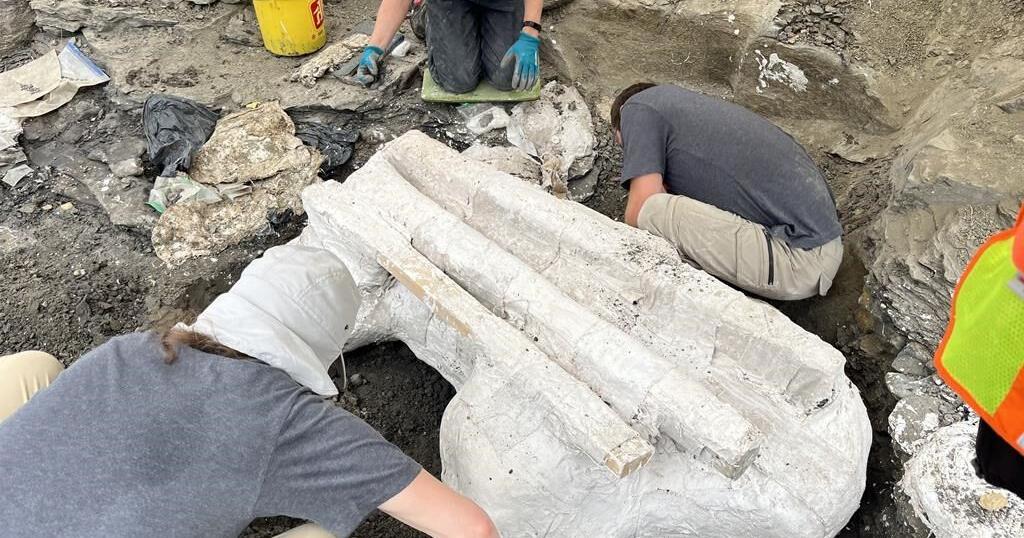
On Wednesday, paleontologists near Grande Prairie pulled its 272-kilogram skull from the ground.
They call it “Big Sam.”
The adult Pachyrhinosaurus is the second plant-eating dinosaur to be unearthed from a dense bonebed belonging to a herd that died together on the edge of a valley that now sits 450 kilometres northwest of Edmonton.
It didn’t die alone.
“We have hundreds of juvenile bones in the bonebed, so we know that there are many babies and some adults among all of the big adults,” Emily Bamforth, a paleontologist with the nearby Philip J. Currie Dinosaur Museum, said in an interview on the way to the dig site.
She described the horned Pachyrhinosaurus as “the smaller, older cousin of the triceratops.”
“This species of dinosaur is endemic to the Grand Prairie area, so it’s found here and nowhere else in the world. They are … kind of about the size of an Indian elephant and a rhino,” she added.
The head alone, she said, is about the size of a baby elephant.
The discovery was a long time coming.
The bonebed was first discovered by a high school teacher out for a walk about 50 years ago. It took the teacher a decade to get anyone from southern Alberta to come to take a look.
“At the time, sort of in the ’70s and ’80s, paleontology in northern Alberta was virtually unknown,” said Bamforth.
When paleontogists eventually got to the site, Bamforth said, they learned “it’s actually one of the densest dinosaur bonebeds in North America.”
“It contains about 100 to 300 bones per square metre,” she said.
Paleontologists have been at the site sporadically ever since, combing through bones belonging to turtles, dinosaurs and lizards. Sixteen years ago, they discovered a large skull of an approximately 30-year-old Pachyrhinosaurus, which is now at the museum.
About a year ago, they found the second adult: Big Sam.
Bamforth said both dinosaurs are believed to have been the elders in the herd.
“Their distinguishing feature is that, instead of having a horn on their nose like a triceratops, they had this big, bony bump called a boss. And they have big, bony bumps over their eyes as well,” she said.
“It makes them look a little strange. It’s the one dinosaur that if you find it, it’s the only possible thing it can be.”
The genders of the two adults are unknown.
Bamforth said the extraction was difficult because Big Sam was intertwined in a cluster of about 300 other bones.
The skull was found upside down, “as if the animal was lying on its back,” but was well preserved, she said.
She said the excavation process involved putting plaster on the skull and wooden planks around if for stability. From there, it was lifted out — very carefully — with a crane, and was to be shipped on a trolley to the museum for study.
“I have extracted skulls in the past. This is probably the biggest one I’ve ever done though,” said Bamforth.
“It’s pretty exciting.”
This report by The Canadian Press was first published Sept. 25, 2024.
TEL AVIV, Israel (AP) — A rare Bronze-Era jar accidentally smashed by a 4-year-old visiting a museum was back on display Wednesday after restoration experts were able to carefully piece the artifact back together.
Last month, a family from northern Israel was visiting the museum when their youngest son tipped over the jar, which smashed into pieces.
Alex Geller, the boy’s father, said his son — the youngest of three — is exceptionally curious, and that the moment he heard the crash, “please let that not be my child” was the first thought that raced through his head.
The jar has been on display at the Hecht Museum in Haifa for 35 years. It was one of the only containers of its size and from that period still complete when it was discovered.
The Bronze Age jar is one of many artifacts exhibited out in the open, part of the Hecht Museum’s vision of letting visitors explore history without glass barriers, said Inbal Rivlin, the director of the museum, which is associated with Haifa University in northern Israel.
It was likely used to hold wine or oil, and dates back to between 2200 and 1500 B.C.
Rivlin and the museum decided to turn the moment, which captured international attention, into a teaching moment, inviting the Geller family back for a special visit and hands-on activity to illustrate the restoration process.
Rivlin added that the incident provided a welcome distraction from the ongoing war in Gaza. “Well, he’s just a kid. So I think that somehow it touches the heart of the people in Israel and around the world,“ said Rivlin.
Roee Shafir, a restoration expert at the museum, said the repairs would be fairly simple, as the pieces were from a single, complete jar. Archaeologists often face the more daunting task of sifting through piles of shards from multiple objects and trying to piece them together.
Experts used 3D technology, hi-resolution videos, and special glue to painstakingly reconstruct the large jar.
Less than two weeks after it broke, the jar went back on display at the museum. The gluing process left small hairline cracks, and a few pieces are missing, but the jar’s impressive size remains.
The only noticeable difference in the exhibit was a new sign reading “please don’t touch.”